In this post I’m going to run through the codes used in R to answer a Bike sharing company’s (Cyclistic) question: How do annual members and casual riders use Cyclistic bikes differently?
I am tasked with the following:
1- Identify how annual cyclists and casual ones use the company’s bikes differently
2- Provide recommendations that will help converting casual riders to annual members
To answer this business question, I’ve completed the following: collect data, wrangle & combine it, cleaning & modifying, conducting decriptive analysis, data vizualization, and finally data exportation.
The public data was collected from Divvy, for a company based in Chicago. Below are the license agreement and data location links:
https://ride.divvybikes.com/data-license-agreement & https://divvy-tripdata.s3.amazonaws.com/index.html
The data used for this project was available in csv format on monthly basis from the period from July-2021 to June-2022. Each month’s data was downloaded and extracted from the zp folder, then uploaded to RStudio path. The csv files are named in this format: yyyymm-divvy-tripdata.csv
to conduct the analysis, the below packages and libraries were installed:
# installing required packages for:

install.packages("tidyverse")     # wrangling data
install.packages("skimr")         # to provide quick descriptive analysis
install.packages("lubridate")     # wrangling data attributes
install.packages("ggplot2")       # for visualization


library(tidyverse)  # wrangle data
library(skimr)      # quick descriptive analysis
library(lubridate)  # wrangle date attributes
library(ggplot2)    # visualize data
library(readr)      # read files
library(dplyr)      # join data frames

getwd()             #displays working directory
STEP 1: Collecting data
The first step was to collect the data from the csv files and add the datasets to the working environment:
# Uploading datasets (csv files)

cyclistic_202107 <- read_csv("202107-divvy-tripdata.csv")
cyclistic_202108 <- read_csv("202108-divvy-tripdata.csv")
cyclistic_202109 <- read_csv("202109-divvy-tripdata.csv")
cyclistic_202110 <- read_csv("202110-divvy-tripdata.csv")
cyclistic_202111 <- read_csv("202111-divvy-tripdata.csv")
cyclistic_202112 <- read_csv("202112-divvy-tripdata.csv")
cyclistic_202201 <- read_csv("202201-divvy-tripdata.csv")
cyclistic_202202 <- read_csv("202202-divvy-tripdata.csv")
cyclistic_202203 <- read_csv("202203-divvy-tripdata.csv")
cyclistic_202204 <- read_csv("202204-divvy-tripdata.csv")
cyclistic_202205 <- read_csv("202205-divvy-tripdata.csv")
cyclistic_202206 <- read_csv("202206-divvy-tripdata.csv")
Then, to ensure that the datasets can be combined into one large datase, the column names and types were checked to ensure that they are matching.
# Comparing column names of each file
# the names don't have to be in order, but they must match *perfectly* to join the data


colnames(cyclistic_202107)
colnames(cyclistic_202108)
colnames(cyclistic_202109)
colnames(cyclistic_202110)
colnames(cyclistic_202111)
colnames(cyclistic_202112)
colnames(cyclistic_202201)
colnames(cyclistic_202202)
colnames(cyclistic_202203)
colnames(cyclistic_202204)
colnames(cyclistic_202205)
colnames(cyclistic_202206)

# all column names match
 >>> [1] "ride_id"            "rideable_type"      "started_at"         "ended_at"           "start_station_name"
     [6] "start_station_id"   "end_station_name"   "end_station_id"     "start_lat"          "start_lng"
    [11] "end_lat"            "end_lng"            "member_casual"
# inspecting data types
str(cyclistic_202107)
str(cyclistic_202108)
str(cyclistic_202109)
str(cyclistic_202110)
str(cyclistic_202111)
str(cyclistic_202112)
str(cyclistic_202201)
str(cyclistic_202202)
str(cyclistic_202203)
str(cyclistic_202204)
str(cyclistic_202205)
str(cyclistic_202206)

# all column data types match

>>> spec_tbl_df [769,204 × 13] (S3: spec_tbl_df/tbl_df/tbl/data.frame)
     $ ride_id           : chr [1:769204] "600CFD130D0FD2A4" "F5E6B5C1682C6464" "B6EB6D27BAD771D2" "C9C320375DE1D5C6" ...
     $ rideable_type     : chr [1:769204] "electric_bike" "electric_bike" "electric_bike" "electric_bike" ...
     $ started_at        : POSIXct[1:769204], format: "2022-06-30 17:27:53" "2022-06-30 18:39:52" "2022-06-30 11:49:25" "2022-06-30 11:15:25" ...
     $ ended_at          : POSIXct[1:769204], format: "2022-06-30 17:35:15" "2022-06-30 18:47:28" "2022-06-30 12:02:54" "2022-06-30 11:19:43" ...
     $ start_station_name: chr [1:769204] NA NA NA NA ...
     $ start_station_id  : chr [1:769204] NA NA NA NA ...
     $ end_station_name  : chr [1:769204] NA NA NA NA ...
     $ end_station_id    : chr [1:769204] NA NA NA NA ...
     $ start_lat         : num [1:769204] 41.9 41.9 41.9 41.8 41.9 ...
     $ start_lng         : num [1:769204] -87.6 -87.6 -87.7 -87.7 -87.6 ...
     $ end_lat           : num [1:769204] 41.9 41.9 41.9 41.8 41.9 ...
     $ end_lng           : num [1:769204] -87.6 -87.6 -87.6 -87.7 -87.6 ...
     $ member_casual     : chr [1:769204] "casual" "casual" "casual" "casual" ...
     - attr(*, "spec")=
      .. cols(
      ..   ride_id = col_character(),
      ..   rideable_type = col_character(),
      ..   started_at = col_datetime(format = ""),
      ..   ended_at = col_datetime(format = ""),
      ..   start_station_name = col_character(),
      ..   start_station_id = col_character(),
      ..   end_station_name = col_character(),
      ..   end_station_id = col_character(),
      ..   start_lat = col_double(),
      ..   start_lng = col_double(),
      ..   end_lat = col_double(),
      ..   end_lng = col_double(),
      ..   member_casual = col_character()
      .. )
     - attr(*, "problems")=<externalptr>
STEP 2: Data wrangling and combining into a single file
to combine the data into one data frame:
# Stacking all monthly data into one big data frame

cyclistic <- bind_rows(                       cyclistic_202107,
                                              cyclistic_202108,
                                              cyclistic_202109,
                                              cyclistic_202110,
                                              cyclistic_202111,
                                              cyclistic_202112,
                                              cyclistic_202201,
                                              cyclistic_202202,
                                              cyclistic_202203,
                                              cyclistic_202204,
                                              cyclistic_202205,
                                              cyclistic_202206)
Checking that the data was combined successfully, the number of rows were compared before and after combinging the data
# to ensure that all rows have been combined the below should return 0

zero_rows = nrow(cyclistic_202107) +
            nrow(cyclistic_202108) +
            nrow(cyclistic_202109) +
            nrow(cyclistic_202110) +
            nrow(cyclistic_202111) +
            nrow(cyclistic_202112) +
            nrow(cyclistic_202201) +
            nrow(cyclistic_202202) +
            nrow(cyclistic_202203) +
            nrow(cyclistic_202204) +
            nrow(cyclistic_202205) +
            nrow(cyclistic_202206) -
            nrow(cyclistic)

print(zero_rows)

  >>> [1] 0
There are some unneessar columns that can be removed without impacting the final outcome:
# longitude and latitude columns won't help answering the business question,
# so it is better to remove them and save space and processing power

cyclistic <- cyclistic %>%
  select(-c(start_lat, start_lng, end_lat, end_lng))
STEP 3: Cleaning and adding data to prepare for analysis
To inspect a newly created table:
colnames(cyclistic)                # List of column names

  >>> [1] "ride_id"            "rideable_type"      "started_at"         "ended_at"           "start_station_name"
      [6] "start_station_id"   "end_station_name"   "end_station_id"     "member_casual"
nrow(cyclistic)                    # How many rows are in data frame?

  >>> [1] 5900385
dim(cyclistic)                     # Dimensions of the data frame?

  >>> [1] 5900385       9
head(cyclistic)                    # See the first 6 rows of data frame.  Also tail(cyclistic)

  >>> # A tibble: 6 × 9
        ride_id        rideable_type started_at          ended_at            start_station_n… start_station_id end_station_name
        <chr>          <chr>         <dttm>              <dttm>              <chr>            <chr>            <chr>
      1 0A1B623926EF4… docked_bike   2021-07-02 14:44:36 2021-07-02 15:19:58 Michigan Ave & … 13001            Halsted St & No…
      2 B2D5583A5A5E7… classic_bike  2021-07-07 16:57:42 2021-07-07 17:16:09 California Ave … 17660            Wood St & Hubba…
      3 6F264597DDBF4… classic_bike  2021-07-25 11:30:55 2021-07-25 11:48:45 Wabash Ave & 16… SL-012           Rush St & Hubba…
      4 379B58EAB20E8… classic_bike  2021-07-08 22:08:30 2021-07-08 22:23:32 California Ave … 17660            Carpenter St & …
      5 6615C1E4EB08E… electric_bike 2021-07-28 16:08:06 2021-07-28 16:27:09 California Ave … 17660            Elizabeth (May)…
      6 62DC2B32872F9… electric_bike 2021-07-29 17:09:08 2021-07-29 17:15:00 California Ave … 17660            Albany Ave & Bl…
      # … with 2 more variables: end_station_id <chr>, member_casual <chr>
str(cyclistic)                     # See list of columns and data types (numeric, character, etc)

  >>> tibble [5,900,385 × 9] (S3: tbl_df/tbl/data.frame)
       $ ride_id           : chr [1:5900385] "0A1B623926EF4E16" "B2D5583A5A5E76EE" "6F264597DDBF427A" "379B58EAB20E8AA5" ...
       $ rideable_type     : chr [1:5900385] "docked_bike" "classic_bike" "classic_bike" "classic_bike" ...
       $ started_at        : POSIXct[1:5900385], format: "2021-07-02 14:44:36" "2021-07-07 16:57:42" "2021-07-25 11:30:55" "2021-07-08 22:08:30" ...
       $ ended_at          : POSIXct[1:5900385], format: "2021-07-02 15:19:58" "2021-07-07 17:16:09" "2021-07-25 11:48:45" "2021-07-08 22:23:32" ...
       $ start_station_name: chr [1:5900385] "Michigan Ave & Washington St" "California Ave & Cortez St" "Wabash Ave & 16th St" "California Ave & Cortez St" ...
       $ start_station_id  : chr [1:5900385] "13001" "17660" "SL-012" "17660" ...
       $ end_station_name  : chr [1:5900385] "Halsted St & North Branch St" "Wood St & Hubbard St" "Rush St & Hubbard St" "Carpenter St & Huron St" ...
       $ end_station_id    : chr [1:5900385] "KA1504000117" "13432" "KA1503000044" "13196" ...
       $ member_casual     : chr [1:5900385] "casual" "casual" "member" "member" ...
skim_without_charts(cyclistic)     # Statistical summary of data

  >>> ── Data Summary ────────────────────────
                                 Values
      Name                       cyclistic
      Number of rows             5900385
      Number of columns          9
      _______________________
      Column type frequency:
        character                7
        POSIXct                  2
      ________________________
      Group variables            None

      ── Variable type: character ─────────────────────────────────────────────────────────────────────────────────────────────
        skim_variable      n_missing complete_rate min max empty n_unique whitespace
      1 ride_id                    0         1      16  16     0  5900385          0
      2 rideable_type              0         1      11  13     0        3          0
      3 start_station_name    836018         0.858   3  64     0     1293          0
      4 start_station_id      836015         0.858   3  44     0     1157          0
      5 end_station_name      892103         0.849   9  64     0     1315          0
      6 end_station_id        892103         0.849   3  44     0     1171          0
      7 member_casual              0         1       6   6     0        2          0

      ── Variable type: POSIXct ───────────────────────────────────────────────────────────────────────────────────────────────
        skim_variable n_missing complete_rate min                 max                 median              n_unique
      1 started_at            0             1 2021-07-01 00:00:22 2022-06-30 23:59:58 2021-10-27 17:35:55  4924385
      2 ended_at              0             1 2021-07-01 00:04:51 2022-07-13 04:21:06 2021-10-27 17:49:46  4924865
Analysis of he above results, we can see that there are:
1- three unique rideable_type
2- many missing station names and id’s
3- two unique values in member_casual
4- the data can only be aggregated at the ride-level, by adding additional columns, such as day, month year, we will have more opportunity to aggregate the data
5- adding ride_length as a calculated field will be beneficial for analysis
By adding columns that list the date, month, day, and year of each ride will allow us to aggregate ride data for each month, day, or year before completing these operations we can only aggregate at the ride level
this link provides more information of data formats in R:
https://www.statmethods.net/input/dates.html
cyclistic$date              <- as.Date(cyclistic$started_at)             # output will be in yyyy-mm-dd
cyclistic$day               <- format(as.Date(cyclistic$date), "%d")     # output will be in range of 01-31
cyclistic$month             <- format(as.Date(cyclistic$date), "%m")     # output will be in range of 01-12
cyclistic$year              <- format(as.Date(cyclistic$date), "%Y")     # output will be in 4-digit year
cyclistic$day_of_week       <- format(as.Date(cyclistic$date), "%A")     # output will be unabbreviated weekday
cyclistic$year_month        <- format(as.Date(cyclistic$date), "%Y-%m")  # output will be in yyyy-mm and will be used to aggregate by month
now, to add the ride length calculation, we use the difftime() function, this will result in a new column with values in unit of seconds, for more details, check out the below link:
https://stat.ethz.ch/R-manual/R-devel/library/base/html/difftime.html
cyclistic$ride_length <-
  difftime(cyclistic$ended_at, cyclistic$started_at)
To check the newly added column, let’s use str() again
>>> str(cyclistic)
    tibble [5,900,385 × 16] (S3: tbl_df/tbl/data.frame)
     $ ride_id           : chr [1:5900385] "0A1B623926EF4E16" "B2D5583A5A5E76EE" "6F264597DDBF427A" "379B58EAB20E8AA5" ...
     $ rideable_type     : chr [1:5900385] "docked_bike" "classic_bike" "classic_bike" "classic_bike" ...
     $ started_at        : POSIXct[1:5900385], format: "2021-07-02 14:44:36" "2021-07-07 16:57:42" "2021-07-25 11:30:55" "2021-07-08 22:08:30" ...
     $ ended_at          : POSIXct[1:5900385], format: "2021-07-02 15:19:58" "2021-07-07 17:16:09" "2021-07-25 11:48:45" "2021-07-08 22:23:32" ...
     $ start_station_name: chr [1:5900385] "Michigan Ave & Washington St" "California Ave & Cortez St" "Wabash Ave & 16th St" "California Ave & Cortez St" ...
     $ start_station_id  : chr [1:5900385] "13001" "17660" "SL-012" "17660" ...
     $ end_station_name  : chr [1:5900385] "Halsted St & North Branch St" "Wood St & Hubbard St" "Rush St & Hubbard St" "Carpenter St & Huron St" ...
     $ end_station_id    : chr [1:5900385] "KA1504000117" "13432" "KA1503000044" "13196" ...
     $ member_casual     : chr [1:5900385] "casual" "casual" "member" "member" ...
     $ date              : Date[1:5900385], format: "2021-07-02" "2021-07-07" "2021-07-25" "2021-07-08" ...
     $ day               : chr [1:5900385] "02" "07" "25" "08" ...
     $ month             : chr [1:5900385] "07" "07" "07" "07" ...
     $ year              : chr [1:5900385] "2021" "2021" "2021" "2021" ...
     $ day_of_week       : chr [1:5900385] "Friday" "Wednesday" "Sunday" "Thursday" ...
     $ year_month        : chr [1:5900385] "2021-07" "2021-07" "2021-07" "2021-07" ...
     $ ride_length       : 'difftime' num [1:5900385] 2122 1107 1070 902 ...
      ..- attr(*, "units")= chr "secs"
Convert “ride_length” from factor to numeric so we can run calculations on the data
is.factor(cyclistic$ride_length)  # returns FALSE
  >>> [1] FALSE
to change from value in seconds to string to numeric value
cyclistic$ride_length <-
  as.numeric(as.character(cyclistic$ride_length))
to check if the conversion was completed correctly
is.numeric(cyclistic$ride_length) # returns TRUE
  >>> [1] TRUE
Let’s check the statistical summary of the ride_length column
skim_without_charts(cyclistic$ride_length)     # Statistical summary of data
  >>> ── Data Summary ────────────────────────
                                 Values
      Name                       cyclistic$ride_length
      Number of rows             5900385
      Number of columns          1
      _______________________
      Column type frequency:
        numeric                  1
      ________________________
      Group variables            None

      ── Variable type: numeric ───────────────────────────────────────────────────────────────────────────────────────────────
        skim_variable n_missing complete_rate  mean    sd    p0 p25 p50  p75    p100
      1 data                  0             1 1217. 9313. -8245 377 670 1212 2946429
we can see that the minimum value in the ride length column is negative, some of the entries in the data frame were when bikes got taken out of docks and checked for quality, we must remove the negative data but it is best to create a new dataframe
cyclistic_v2 <- cyclistic %>%
  filter(ride_length > 0)
STEP 4: Conducting descriptive analysis
descriptive analysis on ride_length (all values in seconds)
mean(cyclistic_v2$ride_length)      #straight average (total ride length / rides)
  >>> [1] 1217.109
median(cyclistic_v2$ride_length)    #midpoint number in the ascending array of ride lengths
  >>> [1] 670
max(cyclistic_v2$ride_length)       #longest ride
  >>> [1] 2946429
min(cyclistic_v2$ride_length)       #shortest ride
  >>> [1] 1
using summary(), the four chunks above can be condensed
summary(cyclistic_v2$ride_length)
   >>> Min. 1st Qu.  Median    Mean 3rd Qu.    Max.
          1     377     670    1217    1212 2946429
it seems that the maximum value is an outlier, and this should be investigated furthur.
to compare members and casual users aggregation fuction was used this link provides examples on how to aggregate:
https://www.statology.org/r-mean-by-group/
average ride length by customer type:
aggregate(cyclistic_v2$ride_length ~ cyclistic_v2$member_casual, FUN = mean)
  >>> cyclistic_v2$member_casual cyclistic_v2$ride_length
    1                     casual                 1789.431
    2                     member                  779.049
median ride length by customer type:
aggregate(cyclistic_v2$ride_length ~ cyclistic_v2$member_casual, FUN = median)
  >>> cyclistic_v2$member_casual cyclistic_v2$ride_length
    1                     casual                      891
    2                     member                      544
max ride length by customer type:
aggregate(cyclistic_v2$ride_length ~ cyclistic_v2$member_casual, FUN = max)
  >>> cyclistic_v2$member_casual cyclistic_v2$ride_length
    1                     casual                  2946429
    2                     member                    93594
min ride length by customer type:
aggregate(cyclistic_v2$ride_length ~ cyclistic_v2$member_casual, FUN = min)
  >>> cyclistic_v2$member_casual cyclistic_v2$ride_length
    1                     casual                        1
    2                     member                        1
to get the average ride time by day of week for members vs casual users, we use the same aggregation function, but add the day of week to the aggregation
aggregate(cyclistic_v2$ride_length, list(cyclistic_v2$member_casual, cyclistic_v2$day_of_week), FUN=mean)

   >>> Group.1   Group.2         x
    1   casual    Friday 1696.1002
    2   member    Friday  763.6394
    3   casual    Monday 1837.7099
    4   member    Monday  758.2602
    5   casual  Saturday 1934.4052
    6   member  Saturday  871.8730
    7   casual    Sunday 2067.6086
    8   member    Sunday  881.4162
    9   casual  Thursday 1634.0557
    10  member  Thursday  747.8117
    11  casual   Tuesday 1544.8222
    12  member   Tuesday  731.5243
    13  casual Wednesday 1544.6104
    14  member Wednesday  732.5412
To organize the days from Sunday to Saturday:
cyclistic_v2$day_of_week <-
  ordered(cyclistic_v2$day_of_week,
          levels=c(   "Sunday",
                      "Monday",
                      "Tuesday",
                      "Wednesday",
                      "Thursday",
                      "Friday",
                      "Saturday"))
Then running the previos code:
aggregate(cyclistic_v2$ride_length, list(cyclistic_v2$member_casual, cyclistic_v2$day_of_week), FUN=mean)

   >>> Group.1   Group.2         x
    1   casual    Sunday 2067.6086
    2   member    Sunday  881.4162
    3   casual    Monday 1837.7099
    4   member    Monday  758.2602
    5   casual   Tuesday 1544.8222
    6   member   Tuesday  731.5243
    7   casual Wednesday 1544.6104
    8   member Wednesday  732.5412
    9   casual  Thursday 1634.0557
    10  member  Thursday  747.8117
    11  casual    Friday 1696.1002
    12  member    Friday  763.6394
    13  casual  Saturday 1934.4052
    14  member  Saturday  871.8730
we can also run this code for the median, maximum and minum ride lengths:
aggregate(cyclistic_v2$ride_length, list(cyclistic_v2$member_casual, cyclistic_v2$day_of_week), FUN=median)

  >>> Group.1   Group.2    x
    1   casual    Sunday 1035
    2   member    Sunday  606
    3   casual    Monday  895
    4   member    Monday  523
    5   casual   Tuesday  780
    6   member   Tuesday  515
    7   casual Wednesday  779
    8   member Wednesday  523
    9   casual  Thursday  792
    10  member  Thursday  528
    11  casual    Friday  847
    12  member    Friday  537
    13  casual  Saturday 1005
    14  member  Saturday  610
aggregate(cyclistic_v2$ride_length, list(cyclistic_v2$member_casual, cyclistic_v2$day_of_week), FUN=max)

   >>> Group.1   Group.2       x
    1   casual    Sunday 2497750
    2   member    Sunday   89996
    3   casual    Monday 1861873
    4   member    Monday   89997
    5   casual   Tuesday 1500471
    6   member   Tuesday   89997
    7   casual Wednesday 2149238
    8   member Wednesday   89998
    9   casual  Thursday 2946429
    10  member  Thursday   89997
    11  casual    Friday 2321116
    12  member    Friday   89998
    13  casual  Saturday 2443476
    14  member  Saturday   93594
aggregate(cyclistic_v2$ride_length, list(cyclistic_v2$member_casual, cyclistic_v2$day_of_week), FUN=min)

   >>> Group.1   Group.2 x
    1   casual    Sunday 1
    2   member    Sunday 1
    3   casual    Monday 1
    4   member    Monday 1
    5   casual   Tuesday 1
    6   member   Tuesday 1
    7   casual Wednesday 1
    8   member Wednesday 1
    9   casual  Thursday 1
    10  member  Thursday 1
    11  casual    Friday 1
    12  member    Friday 1
    13  casual  Saturday 1
    14  member  Saturday 1
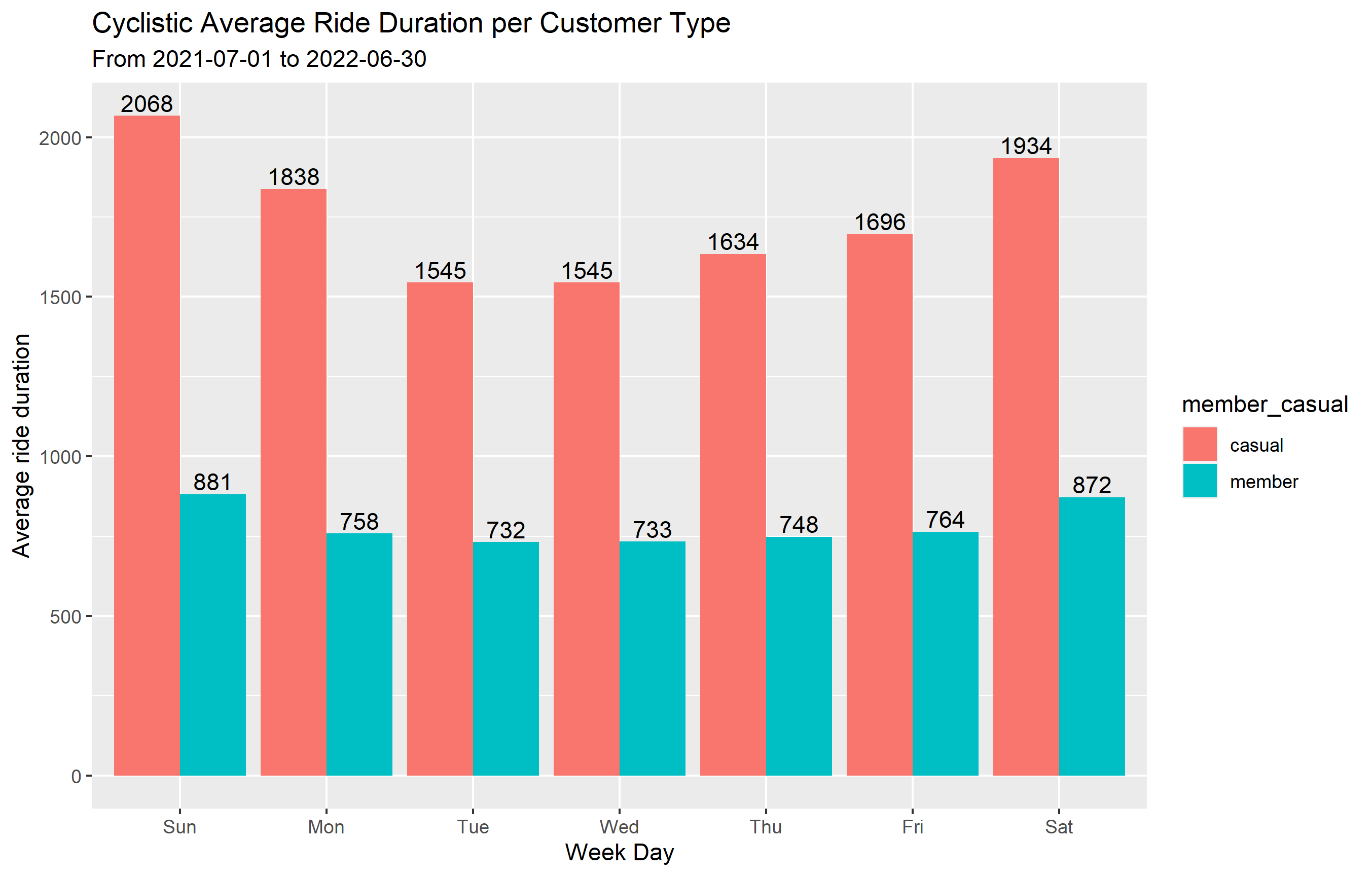
The statistical analysis shows that on any given day, casual riders have longer trips than annual memebers.
Let’s create new datasets that show the number of rides and average ride length per day of week and another per month from the start to end of the dataset (2021-07-01 to 2022-06-30) for each customer type:
weekday data:
summarized_data <- cyclistic_v2 %>%
  mutate(weekday = wday(started_at, label = TRUE)) %>%    #creates weekday field using wday() True gives day name
  group_by(member_casual, weekday) %>%                    #groups by usertype and weekday
  summarize(number_of_rides = n()							            #calculates the number of rides and average duration
            ,average_duration = mean(ride_length)) %>% 		# calculates the average duration
  arrange(member_casual, weekday)							          	# sorts

 >>> `summarise()` has grouped output by 'member_casual'. You can override using the `.groups` argument.

 print(summarized_data)
 >>> # A tibble: 14 × 4
    # Groups:   member_casual [2]
       member_casual weekday number_of_rides average_duration
       <chr>         <ord>             <int>            <dbl>
     1 casual        Sun              467027            2068.
     2 casual        Mon              303967            1838.
     3 casual        Tue              277738            1545.
     4 casual        Wed              285450            1545.
     5 casual        Thu              325143            1634.
     6 casual        Fri              363065            1696.
     7 casual        Sat              535497            1934.
     8 member        Sun              398881             881.
     9 member        Mon              469011             758.
    10 member        Tue              518207             732.
    11 member        Wed              516507             733.
    12 member        Thu              525901             748.
    13 member        Fri              469221             764.
    14 member        Sat              444124             872.
monthly data:
summarized_month <- cyclistic_v2 %>%
  group_by(member_casual, year_month) %>%                      #groups by usertype and month
  summarize(number_of_rides = n()							            #calculates the number of rides and average duration
            ,average_duration = mean(ride_length)) %>% 		# calculates the average duration
  arrange(member_casual, year_month)							                  	# sorts

>>> `summarise()` has grouped output by 'member_casual'. You can override using the `.groups` argument.

>>> print(summarized_month)
    # A tibble: 24 × 4
    # Groups:   member_casual [2]
       member_casual year_month number_of_rides average_duration
       <chr>         <chr>                <int>            <dbl>
     1 casual        2021-07             442011            1968.
     2 casual        2021-08             412608            1727.
     3 casual        2021-09             363840            1669.
     4 casual        2021-10             257203            1721.
     5 casual        2021-11             106884            1388.
     6 casual        2021-12              69729            1410.
     7 casual        2022-01              18517            1823.
     8 casual        2022-02              21414            1603.
     9 casual        2022-03              89874            1958.
    10 casual        2022-04             126398            1772.
    # … with 14 more rows
we can export these datasets for vizualization and analysis.
STEP 5: Export summarized data for further analysis
by creating a csv file, we can export the data out of R and use it on Tablaue, excel or any other data viz tool
write.csv(summarized_weekday,
          "C:/"Enter your path and file name".csv",
          row.names = TRUE)


write.csv(summarized_month,
          "C:/"Enter your path and file name".csv",
          row.names = TRUE)
Data visualization
To create data visualizations using R, for week day and monthly data, the following codes were used:
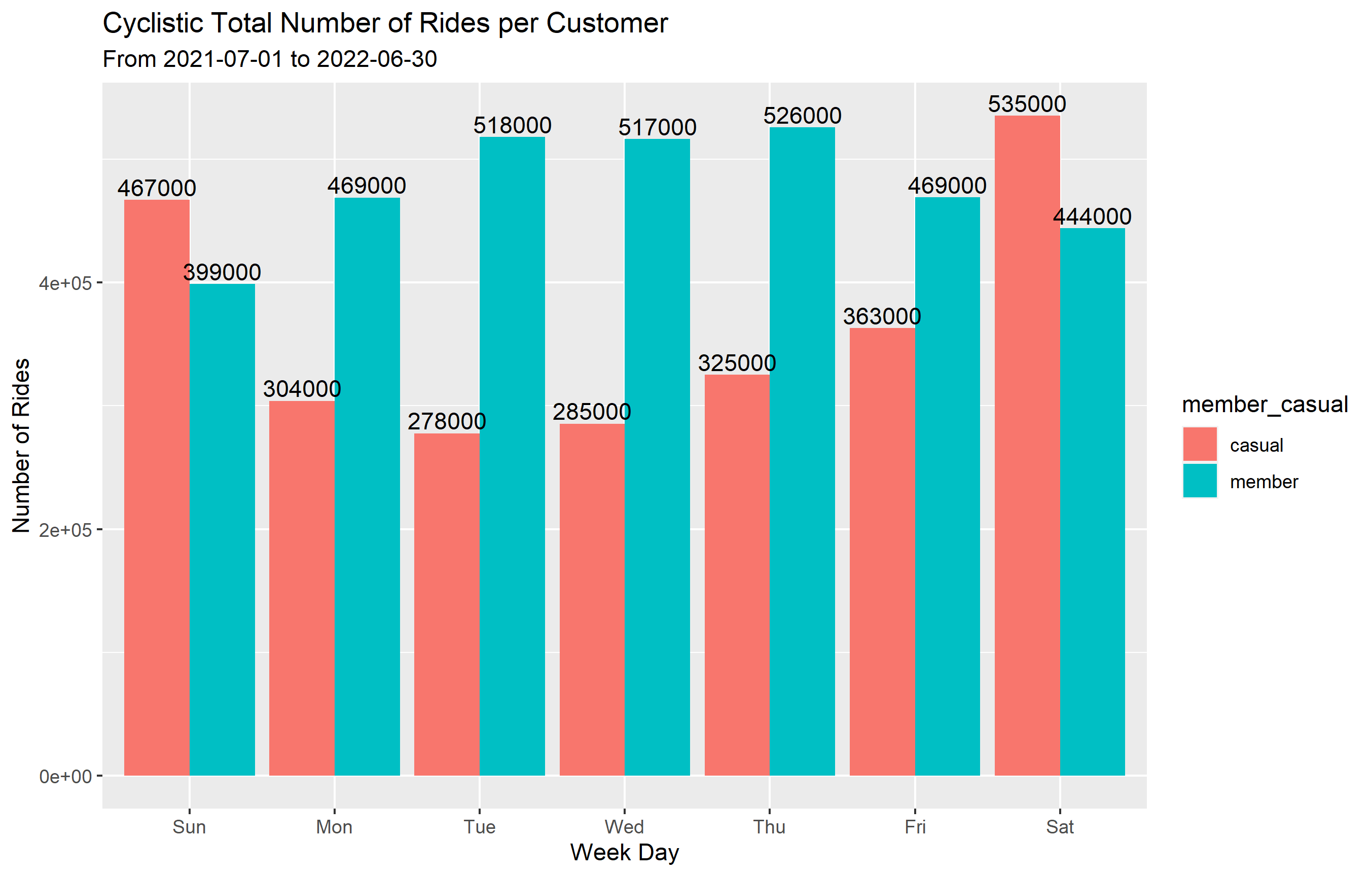
summarized_weekday %>%
  ggplot(aes(x = weekday,                                       # x-axis is weekdays
             y = number_of_rides,                               # y-axis is number of rides
             fill = member_casual)) +                           # fill columns by customer type
  geom_col(position = "dodge") +                                # separate bar for each customer type instead of stacked
  labs(title = "Cyclistic Total Number of Rides per Customer",  # plot title
     subtitle = "From 2021-07-01 to 2022-06-30",                # plot subtitle
     y= "Number of Rides",                                      # y-axis label
     x = "Week Day") +                                          # x-axis label
  geom_text(aes(label = round(number_of_rides,-3)),             # add number of rides to the plot rounded to the nearest thousand
            position = position_dodge(width = 0.9),             # positioning and colouring functions
            vjust = -0.25, color = "black")

ggsave("Number of Rides per Customer-weekday .png")             # save plot as
summarized_weekday %>%
  ggplot(aes(x = weekday,                                           # x-axis is weekdays
             y = average_duration,                                  # y-axis is number of rides
             fill = member_casual)) +                               # fill columns by customer type
  geom_col(position = "dodge") +                                    # separate bar for each customer type instead of stacked
  labs(title = "Cyclistic Average Ride Duration per Customer Type", # plot title
       subtitle = "From 2021-07-01 to 2022-06-30",                  # plot subtitle
       y= "Average ride duration",                                  # y-axis label
       x = "Week Day") +                                            # x-axis label
  geom_text(aes(label = round(average_duration, 0)),                # add number of rides to the plot rounded to the nearest whole number
            position = position_dodge(width = 0.9),                 # positioning and colouring functions
            vjust = -0.25, color = "black")

ggsave("Average Ride Duration per Customer Type-weekday .png")             # save plot as
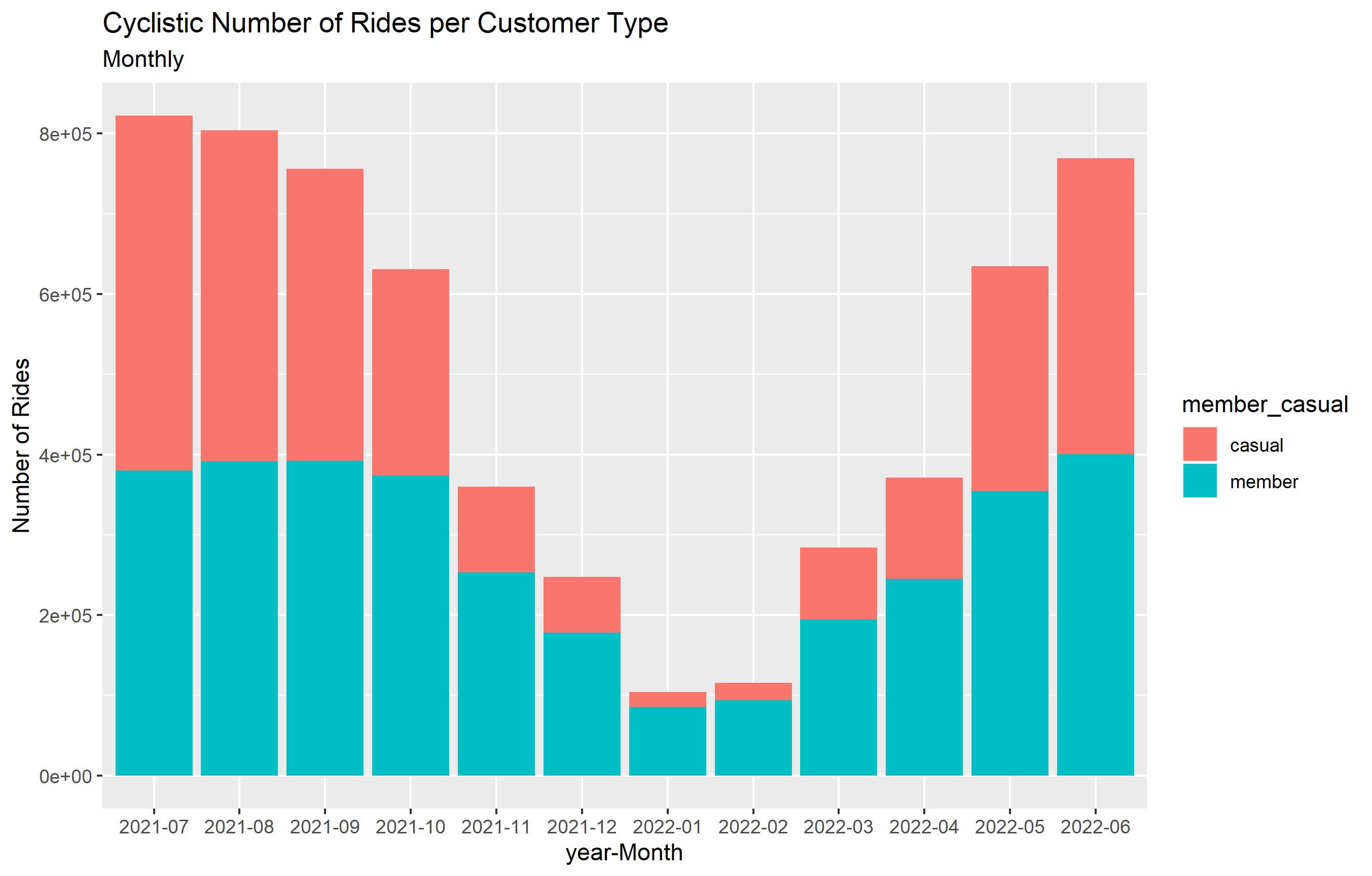
  ggplot(data = summarized_month) +
  geom_col(mapping = aes(x = year_month,
                          y = number_of_rides,
                          fill = member_casual)) +
  labs(title = "Cyclistic Number of Rides per Customer Type", # plot title
       subtitle = "Monthly",                  # plot subtitle
       y = "Number of Rides",
       x = "year-Month")

ggsave("Number of Rides per Customer Type-Monthly .png")             # save plot as
ggplot(data = summarized_month) +
  geom_point(mapping = aes(x = year_month,
                         y = average_duration,
                         color = member_casual,
                         size = 3)) +
  labs(title = "Cyclistic Number of Rides per Customer Type", # plot title
       subtitle = "Monthly",                  # plot subtitle
       y = "Number of Rides",
       x = "year-Month")

ggsave("Average Ride Duration per Customer Type-Monthly .png")             # save plot as

After the analysis and visualization, these are my recomendations to convert casual riders to annual customers:
1- Provide a weekly or monthly subscription trial for casual riders and share with them a visualization on the savings they can make by joining the annual membership, instead of paying per ride.
2- The number of bike rides drops significantly during winter months and starts to go higher by the end of February, this provides a great chance for the company to sart advertising post winter to attract more customers.
3- The data shows that casual customers have a higher ride duration than annaual riders on days of the week and also on monthly basis, therefore the company can set a cap on the length of time they can use the bike brfore being charged an extra amount. This will not apply to annual members and may help in converting customers.